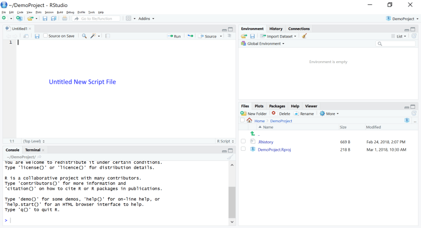
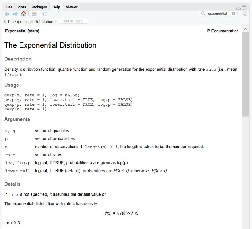
In the last post I talked about how to save and reuse code and commands in RStudio. I included the below screenshot of the workspace in RStudio, with the panes labeled.

Now we will focus on the top right pane, where it says “Import and examine data here”.

Importing a Comma Separated Text File

But first we need data to import. I will cover creating a data file in another post, so let’s assume we have a data file created in Excel and saved as a CSV file (comma-separated values) file. This data file contains 7 columns containing the number of plain M&Ms from two fun sized packs as well as the number in each color. Partial M&Ms were rounded up to the next whole number.

To import this data, in the Environment tab, click on Import Dataset (or go to File > Import Dataset). You will notice there are several options. For a CSV file there are two options that will work. Either From Text (base)… or From Text (readr)… I will not go into the technical details of the differences between the two options, but essentially after importing they store the data in different formats.

Import CSV using From Text (base)…

The traditional way of importing data from text files into R is using this base package import tool. After selecting this option, a file browser will open to allow you to select the file to import. Below is how the dialog looks after selecting the M&M data file.

Notice the weird characters and the column of undefined values. Unfortunately, this is a problem with creating files in Excel and importing using the From Text (base)… option. One of the great things about RStudio is that you get a preview of what your data will look like before you import it. This should prevent the problem of importing the data and then later realizing that something went wrong on the import step. It is also fortunate that we have a great tool available to fix this issue! We will open the text file in RStudio, edit it and then try to import again. So select Cancel.

From the File menu, select File > Open File… and select that same file to open. Note, this step does not import data!

If you see any weird characters you didn’t intend, delete them. Even if the data looks perfectly fine (as in this case), we want to save this file as a new copy. So go to File > Save As… and give the file a new name.

Then go back to the Import Dataset… option and select From Text (base)… again. Even though the only thing we did was open in R and saved a new copy of the file, now the preview of the data looks much better. Make sure, if you have headers (n, Yellow, etc.) that the Heading option on the left says Yes.

After clicking Import, the data will be imported and loaded into the environment and opened in a view tab. The code used to import the data will be printed in the console. You can copy this code and save it at the beginning of a script so that you don’t have to manually go through the import process if you close the RStudio session before you are done.

The biggest issue with using From Text (base)… is that it has a problem handling files opened in Excel, but it is better at importing datasets that have factor variables.

Here is another dataset example, this time the file is a tab delimited text file:

When importing this into RStudio using From Text (base)…, you can preview the variables by clicking on the blue arrow button in the Environment pane.

You can see that Sex is listed as a Factor variable, meaning it is a categorical variable with two levels (“M” and “F”).

Import CSV using From Text (readr)…

There is an alternate package that imports text files. It generally handles files opened in Excel better but does not automatically classify variables as Factors.

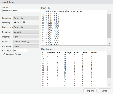
To use this data importer, click on the From Text (readr)… option. You will notice that instead of opening a file explorer you see the Import Text Data window below.

Click on the Browse… button to select the file.

First, we will look at the M&M Data again. I have selected the file that was opened in Excel that did not look right when using the other data import option. You can see here that it looks fine.

To finish the import, click Import.

Now, let’s import the bears data. Note that initially it doesn’t look good. That is because this data importer cannot automatically detect the delimiter in the file and it is set to comma by default.

 

Click in the drop down menu for Delimiter and change it to Tab. Now the columns/variables should be automatically detected and it should look good other than the fact that Sex is identified as a categorical variable. You can change this to a factor variable in this data view, but you have to know all of your factor level values exactly which might not always be the case. So I prefer to fix it after import.

When you are ready to import, click Import.

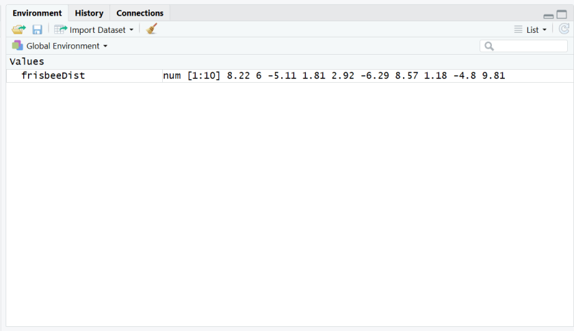
Above is what the data looks like in the Environment pane after importing using From Text (readr)…. Note that Sex is identified as a “chr” variable type.

To change Sex to a factor variable we just need to run one line of code. Remember the code from the import and factor conversion process can be saved in an R script for reuse later and you can run all of this at once the next time you open RStudio.

To convert to a factor use this line of code:

BearsData$Sex <- as.factor(BearsData$Sex)

See how that changes the Environment Pane for the BearsData:

So there are pros and cons to each method of importing data from text files. There are other options available for importing data into R and RStudio, but these are the two primary commands you will use.

What’s Next?

The next blog post will cover how to use Excel to take raw data from scraps of paper to create a file to import into RStudio for analysis.

If you have any questions please don’t hesitate to reach out to greatlineswriting@outlook.com!

When trying to complete an assignment or a complicated analysis all of the work cannot be completed in one sitting. Even if it could, you should want to have a record of what you did in case you need to rerun the analysis or use it again for a similar but different situation. To do this we can use R script files. RStudio makes it straight forward to do this, you can even just use a script as a scratch space without formally creating a file.

In this post, I’ll walk you through adding this capability to your RStudio workspace and some short cuts and tricks to using scripts.

Adding a script file to your RStudio view

Just a reminder, your workspace should look like the below view if you haven’t already opened a file or a script in RStudio:

To add a script file, either click on the green plus button on the upper left in the tool bar and select R Script or go to File > New File > R Script or on Windows use the commands Ctrl + Shift + N. On Mac OS this should be Command + Shift + N.

After you add the script your RStudio view should look like the following (a new pane is added to the upper left):

Everything that we can type in the Console we can type in the Script file, the only difference is that you won’t see a carat at the beginning of the line. In a script file you can run one line of code at a time or multiple lines.

Running commands from a script file

In my previous post (Learning How to Use RStudio as a Calculator) we created a variable and calculated some summary statistics on the data. Let’s use these data again now in a script.

In the script file, copy and paste the following (copy all 4 lines at once):

frisbeeDist <-c(8.22,6.00,-5.11,1.81,2.92,-6.29,8.57,1.18,-4.80,9.81)
mean(frisbeeDist)
sd(frisbeeDist)
summary(frisbeeDist)

Your script file should look like this:

We will start by running one line of code at a time. Click anywhere in the first line where we are saving the data to the frisbeeDist variable. There are a few ways to run or perform this action.

To run a line of code perform one of the following actions:

1. Click on the Run button on the upper right of the script window.
2. Use the command Ctrl + Enter on Windows or Command + Return on Mac OS.
3. From the Code menu, select, Run Selected Line(s).

After you run the first line, it will be automatically copied to the Console and the command executed. All output will be in the Console.

Similarly the next three lines of code can be run one line at a time, or you can highlight all three lines and run all three at once. The actions are performed from top down so that if a line depends on a line above the actions will be performed in the correct order.

Once you select the lines, use one of the three ways to run code as listed above. The resulting Console window will look like this:

Adding Comments to a Script File

The whole point of using script files is to keep code that you have run so that you can reuse it at a later time. In order to really take advantage of that you need to leave yourself notes as to what you did and why. You can do this in R Scripts by indicating a line is a comment and not something that should be executed.

We indicate a line in a script is a comment by starting the line with at least one hash or pound symbol: #. Commented lines will be green in the script file. In the image below I have added comments to the previous lines of files. Note these comments are copied to the console but no action is taken and are blue in the console.

One other trick to making your files readable is adding white lines or spaces to break up the content. White lines when executed just act as a return in the console and just add blank lines between previous code or output and the next line of code or output.

Question: Which script file is more readable and understandable?

Saving the file

Now, you can take advantage of RStudio automatically saving and remembering anything typed in a script file and just close RStudio without saving this script to a named file. However, if anything happened to your computer you run the risk of losing this information. So I strongly recommend having a single script file for an assignment or project. To save the script, you can either click on the blue save icon, use the keyboard commands Ctrl + S on Windows or Command + S on Mac OS or go to File > Save. This file will be open in RStudio the next time you reopen RStudio unless you click on the X on the file tab to close it.

Viewing other files or data in RStudio

Many other types of files can be opened in RStudio besides RScripts. All of these files or data views will be created as tabs in this upper left hand pane. I will discuss importing data into RStudio in my next blog post, once data is imported, if you view the file it will be available as a tab.

Here is what it will look like to view data in a tab (with the previous script saved as “frisbeeDistAnalysis.R”:

What’s Next?

The blog post will cover how to import data into RStudio to do analysis on sample data.

If you have any questions please don’t hesitate to reach out to greatlineswriting@outlook.com!

 

Now that you have R and RStudio installed, I will show you how to use the software by first starting with the basics of just using RStudio as a fancy calculator. It is a much nicer calculator than a hand held calculator as it can provide help and feedback to make sure you are running the correct commands.

I am going to structure the blog post assuming that you are following along and running the commands in RStudio as we go.

After installing RStudio and launching the application you should see something that looks like this:

Let’s get started!

RStudio R Console

The first thing you should notice in the Console is the version of R you are running. R likes to name their versions interesting names. The version this post is based on is “Kite-Eating Tree” aka version 3.4.3. If you have a different version than someone else it is possible that your results may be different than the other person, but that is generally not the case with basic functions, the focus of this blog post.

Let’s start out by calculating the mean of 10 numbers the “long” way or formula based way in R.

After the greater than symbol ( > ) in the Console type the following:

8.22 + 6.00 + -5.11 + 1.81 + 2.92 + -6.29 + 8.57 + 1.18 + -4.80 + 9.81

Hint, you can copy and paste it the above line! After pasting it, hit enter. You should see the following:

Now of course, that is not the mean but the sum of the 10 values, to find the mean we need to divide by 10. So we can divide 22.31 by 10:

22.31 / 10

Which gives us:

Now, let’s say we want to get more statistics on those 10 numbers. Then we really want to save them as a list of values in a variable that we can refer back to for various calculations.

When creating variable names you want to give it an informative name. Let’s say that these values represent the distance a Frisbee lands from a target. It could fall short or go too far. In this case, it looks like most went too far. So let’s name the variable “frisbeeDist”.

We will store the data in a vector using the R function “c( )” which means we will combine all of the values. The symbols “<-” means we are storing the values in that variable name.

frisbeeDist <-c(8.22,6.00,-5.11,1.81,2.92,-6.29,8.57,1.18,-4.80,9.81)

Once you create a variable it looks like nothing happened, but if you check the Environment tab, you should see the variable and its values.

We can use this variable now to calculate the mean and the standard deviation of this data. The command to calculate a mean of a variable is “mean(x)” where x is the variable name. The command to calculate the standard deviation of a variable is “sd(x)” where x is the variable name. Here are those commands using the data stored in the frisbeeDist variable.

mean(frisbeeDist)
sd(frisbeeDist)

Using RStudio to calculate probabilities

In statistics, we generally no longer use tables to look up probabilities for distributions and we would prefer not to calculate discrete probabilities by hand if the distribution of the data is a named distribution.

Commands for Families of Discrete Random Variables

Let’s start with the binomial distribution. This is a distribution for a discrete random variable so we can compute the probability that X is a specific number as well as the cumulative probabilities.

In R to find the probability that X takes on a certain number we will use the function “dbinom(x, size, probability)”. The “d” stands for density or mass of the probability at that value of x.

To find the cumulative probability that X takes on all values up to and including a particular value we will use the function “pbinom(x, size, probability)”. The “p” stands for distribution function.

Example: Each of 6 randomly selected soda drinkers is given a glass containing Coke and a glass containing Pepsi. The glasses are identical except for a code on the bottom to ID the drink. Suppose the tendency among soda drinkers to prefer Coke to Pepsi is 60%. Let X= the number among the 6 who prefer Coke.

What is the probability that exactly 3 people prefer Coke?

To find this we want to find P(X=3), so our x value is 3, the sample size is 6, and the probability is 0.60 and we use “dbinom”. Run the following code to find the probability.

dbinom(3, 6, 0.6)

Answer: P(X=3) = 0.276

What is the probability that at most 3 people prefer Coke?

To find this we want to find P(X ≤ 3), so the x value is still 3, the sample size is 6, and the probability is 0.60 and we use “pbinom”. Run the following code to find the probability.

pbinom(3, 6, 0.6)

Answer: P(X ≤ 3)=0.4557

There are similar commands for hypergeometric, negative binomial, Poisson, and other discrete random variable distribution families.

Commands for Families of Continuous Random Variables

For continuous random variables it does not make sense to compute a probability at a point as that will always be zero. However the cumulative density function is of great importance. This function is still prefaced with a “p”. Also of interest is calculating percentiles of distributions. This is prefaced with a “q” which stands for quantile. R could not use “p” as it was already taken for the cumulative density function.

To consider these commands, let’s take the normal distribution. The command for a probability that X takes on all values up to and including a certain value is given by the command “pnorm(x, mean, standard deviation)”. To find the percentile or value of x that results in a certain probability to the left of the unknown x we use the command “qnorm(probability, mean, standard deviation)”.

Example: Suppose that adult male polar bears weigh on average 370 kg with a standard deviation of 88 kg.

What is the probability that a randomly selected adult male polar bear will weigh less than or equal to 355 kg?

To find this we want to find P(X ≤ 355), so the x value is 355, the mean is 370 and the standard deviation is 88.

pnorm(355, 370, 88)

Answer: P(X <= 355) = 0.4323 or 43.23%

What weight of adult male polar bears corresponds to the 35th percentile?

To find this we want to find x such that P(X ≤ x) = 0.35, so the probability is 0.35, the mean is 370 and the standard deviation is 88.

qnorm(0.35, 370, 88)

Answer: 35% of adult male polar bears will weigh less than 336.09 kg.

There are similar commands for exponential, gamma, beta, chi-squared and other continuous random variable distribution families.

Getting help on R Commands in RStudio

On the lower right hand side of the RStudio window there are 5 tabs, Files, Plots, Packages, Help, and Viewer. If you click on the Help tab there is a search box. In that box you can either type a search string or a command name if you know it.

If you type a search string it will bring up results from various sources. When getting started with R you will most likely want any solutions that are in the base package or in the stats package so prefer results that have “base::” or “stats::” in front of them.

If you click on the “stats::Exponential” link it brings you to a help page for that topic:

What’s Next?

The next two blog posts will cover how to save and re-use commands in R scripts (and why you might want to do that) and how to import data into RStudio to do analysis on sample data.

If you have any questions please don’t hesitate to reach out to greatlineswriting@outlook.com!

If you are reading this post then you are tasked with learning how to use R and/or RStudio to perform statistics. Either you are a student who is told that you must use RStudio for class or you are someone who has a statistical question you want an answer for (either for yourself or someone else) and want to know how to get the answer without spending a lot of time and money to get it.

R is a great language to answer statistical questions. The base language has been around for quite some time (around 1997, see https://cran.r-project.org/doc/FAQ/R-FAQ.html) and is designed to allow anyone to write instructions to perform specific actions (called packages) which are generally freely downloadable and can be used by anyone. If you are curious about the history of R as a programming language the Wikipedia page is also a good place to start (https://en.wikipedia.org/wiki/R_(programming_language) ). The history is not important for the purposes of this blog post.

Operating System Identification

One of the most important things you need to do before starting to work with R is identify your operating system as it will change what you will download and install on your computer. If you are a computer novice there are three major operating systems: Windows, Mac, and Linux.

If you don’t know if you have a Linux operating system, unless you are borrowing someone else’s computer, then the chances of you having a Linux computer are small. Ok, unless you have a Chrome Book. If so, unfortunately you will need to find a different computer to use, as R and RStudio will not run on a Chrome Book.

If you don’t know if you have a Windows or Mac computer, you will know it is Windows if you see a Windows icon on the task bar (https://en.wikipedia.org/wiki/Taskbar). If you have an apple on the end of the menu bar (https://en.wikipedia.org/wiki/Menu_bar) or have a keyboard button that says “Command” then you have a Mac OS X operating system.

Mac OS X Version

To find out what version of the Mac operating system you have, click on the apple and select “About this Mac” you will want to find the version number, it should start with 10 and be something like 10.6.4 or 10.13.1. You will need to make sure to make the correct choice for the software to download and install. Don’t worry, I’ll walk you through that choice.

First — Install R

To use RStudio (which I highly recommend for the novice statistician or student) you will first need to download and install the R software language and base package. Then we will install RStudio which will make your user experience much friendlier. At this point there will continue to be two sets of instructions, one for Windows and one for Mac OS X.

Windows OS

Go to https://cran.r-project.org/bin/windows/base/ and click on the top link which will be something like “Download R 3.4.3 for Windows”. After clicking on the link, a pop-up window will appear, click on Save File:

This will save the installer to your computer in the location where your downloads go. Depending on your web browser, it is often easier to access the file from the web browser instead of the Downloads folder. In Mozilla Firefox clicking on an arrow pointing down is how you access the recent downloads. On Chrome the file is available at the bottom of the window.

Click on the file to run the installer.

You may need to grant permission to have the installer run. Give permission. If you are told you do not have the required permission needed to run the installer you will need to talk to whomever has administrative control over your computer.

The first option will ask what language you will want to use during installation. It is highly recommended that you select a language that you are both comfortable with as well as the language of choice of whomever you may ask for installation assistance from.

The next screen is the software license. R is licensed under GNU General Public License. Once you have read the license agreement, click Next >.

Unless you have a strong reason to change the installation location, keep the default on the next screen and click Next > again.

Continue to click next until you get to the screen that lists “Select Additional Tasks”. Make sure you keep both registry options checked but you can change the selections for the shortcuts. I strongly recommend unchecking the desktop shortcut option because the shortcut only launches R not RStudio. So you should never need to launch R. After you click Next > R will install.

If it all worked as it should then you should see a screen like the one below. Click Finish.

Now you are ready to install RStudio.

Mac OS X

At the time of this blog post there are three different options for installers (https://cran.r-project.org/bin/macosx/) depending on your Mac OS X version. If you do not have a current operating system you will not have access to the latest versions of R but it is still usable for most purposes for the beginner statistician and student.

If your Mac OS X version is between 10.6 and 10.8.5 you will want to download the Snow Leopard installer: https://cran.r-project.org/bin/macosx/R-3.2.1-snowleopard.pkg.

If your Mac OS X version is between 10.9 and 10.10.5 you will want to download this installer: https://cran.r-project.org/bin/macosx/R-3.3.3.pkg.

If your Mac OS X version is greater than 10.11 then you can download the latest version of R which should always be the top link. At this time, the link for the current version is https://cran.r-project.org/bin/macosx/R-3.4.3.pkg but this link will soon be out of date as there are at least 3 new versions of R released a year.

I am unable to provide screenshots of the installation process on Mac OS X as I do not have access to a Mac computer, however, the installation follows the basic installation of any new package on Mac. After downloading, in the downloads folder click on the package and drag the package icon into your Apps folder.

Now we are ready to install RStudio.

Second — Install RStudio

Windows OS

RStudio is a commercial company that provides an easier to use interface for the R language. This interface is free for most users (including students). Most people will want to select the “Open Source Edition” for the “Desktop”. The link to the latest installers is: https://www.rstudio.com/products/rstudio/download/#download. You will need to remember your operating system from above to select the correct option.

The current link to the Windows installer is: https://download1.rstudio.org/RStudio-1.1.383.exe.

The current link to the Mac OS X installer is: https://download1.rstudio.org/RStudio-1.1.383.dmg. Note for Mac OS X there is only one installer as long as your operating system is 10.6 or newer.

Once you click on the link the installer will download. Click “Save File” or the equivalent option for your web browser. Again, once it is downloaded, access the installer either from your web browser recent downloads list or from the folder where your downloads are stored on your computer.

Run the installer. On Windows this is what the installer will look like:

Click Next > through all of the options and it will start to install. When it is done the installer will show the finished page.

Click Finish.

*Important* Nothing will happen but RStudio will be installed.

Launching RStudio

Mac OS X

On Mac OS X the application will be in your Applications folder. I strongly recommend pinning it to your dock. You can do this by opening the application from the Applications folder. Then right-click on the icon in the dock and select “Keep in Dock”.

Now RStudio is ready to use and easily accessible for the future.

Windows OS

On Windows there may be a desktop icon (if you didn’t uncheck that option from the additional tasks step of the installer). This is not the icon to launch RStudio. Do not use this icon.

I find the easiest way to launch applications is on Windows 10 to type the application in the search bar on the tool bar “RStudio” or using the keyboard press the Windows key next to the Alt key and then type in RStudio. On Windows 7, if you click on the Windows menu on the tool bar there should be a search option available.

Type RStudio in the search box.

Select RStudio and it will launch.

The first time you launch RStudio this is what you will see:

Next…

Now that you have RStudio installed you will want to get started using it! The next blog post will cover an orientation to what you can see in the image above as well as how to start running basic statistics and how to get help when you need it.

If you have any suggestions about topics you would like me to cover please feel free to reach out to greatlineswriting@outlook.com.